HW3 Cheatsheet

Transfer Functions

Zeroes and Poles

Suppose that we represent a transfer function as:

$$H(z)=\frac{N(z)}{D(z)}$$

To find the zeroes of a transfer function, solve for $z$ such that

$$N(z)=0.$$

Similarly, to find the poles of a transfer function, solve for $z$ such that

$$D(z)=0.$$

Solving for roots in polynomials may result in complex and/or repeated roots.

Factoring roots with NumPy

import numpy as np
 
coeffs = [1, -0.25, -1, -1.2]
roots = np.roots(coeffs)
print(roots)

Plotting roots with matplotlib

import matplotlib.pyplot as plt
 
fig, ax = plt.subplots(figsize=(5,5))
 
# draw unit circle
theta = np.linspace(0, 2*np.pi, 400)
ax.plot(np.cos(theta), np.sin(theta))
 
# plot roots
ax.scatter(roots.real, roots.imag, marker='o')
 
# set up axes
ax.axhline(0)
ax.axvline(0)
ax.set_aspect('equal', adjustable='box')
ax.set_xlabel('Re')
ax.set_ylabel('Im')
plt.tight_layout()
plt.show()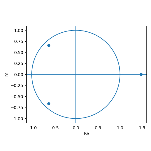

First-Difference Filters

Impulse Function:

$$h[n]=\delta [n]-\delta [n-1]$$

Transfer Function:

$$H(z)=1-z^{-1}=\frac{z-1}{z}$$

Cascaded First-Difference Filters Example

Find the transfer function for a third-order cascade of first-difference filters.

The transfer function for a single first-difference filter is $H_1(z)=1-z^{-1}$ . To cascade this filter, we multiply it by itself. Thus,

$$H(z)=(1-z^{-1}{)}^3=1-3z^{-1}+3z^{-2}-z^{-3}$$

Alternatively, if we represent the first-difference filter transfer function as $H_1(z)=\frac{z-1}{z}$, then:

$$H(z)={\left(\frac{z-1}{z}\right)}^3=\frac{(z-1{)}^3}{z^3}$$

This fraction form makes it easier to find the zeroes and pole of the filter.

Inverse Z-transforms

Properties

Linearity

If $X(z)\stackrel{{\mathcal{Z}}^{-1}}{\leftrightarrow }x[n]$ and $Y(z)\stackrel{{\mathcal{Z}}^{-1}}{\leftrightarrow }y[n]$, then:

$$aX(z)+bY(z)\stackrel{{\mathcal{Z}}^{-1}}{\leftrightarrow }ax[n]+by[n].$$

Time-Shifting

$$z^{-k}X(z)\stackrel{{\mathcal{Z}}^{-1}}{\leftrightarrow }x[n-k]$$

Transforms to Know

Polynomial

$$z^{-k}\stackrel{{\mathcal{Z}}^{-1}}{\leftrightarrow }\delta [n-k]$$

Proof

Recall that the equation for Z-transforms is given by:
$X(z)=\sum _{n=-\infty }^{\infty }x[n]z^{-n}$
Then, if $x[n]=\delta [n-k]$,

$$\begin{array}{rl}X(z)& =\sum _{n=-\infty }^{\infty }\delta [n-k]z^{-n}\\ & =z^{-k}\end{array}$$

Polynomial Example

Find the impulse function for $X(z)=3+4z^{-2}-6z^{-5}$.
Using $z^{-k}\stackrel{{\mathcal{Z}}^{-1}}{\leftrightarrow }\delta [n-k]$:

$$\boxed{x[n]=3\delta [n]+4\delta [n-2]-6\delta [n-5]}$$

Geometric Series

$$\frac{1}{1-a{z}^{-1}}\stackrel{{\mathcal{Z}}^{-1}}{\leftrightarrow }{a}^{n}u[n],\text{ROC: }|z|>|a|$$

Geometric Series Example

Find the impulse function for the system $y[n]=\frac{1}{4}y[n-1]+\frac{1}{8}y[n-2]+x[n]-2x[n-1]$ .
We start off by putting the equation in standard form:

$$y[n]-\frac{1}{4}y[n-1]-\frac{1}{8}y[n-2]=x[n]-2x[n-1].$$

Then, using Z-transform’s time-shifting property $z^{-k}X(z)\stackrel{{\mathcal{Z}}^{-1}}{\leftrightarrow }x[n-k]$, the equation can be represented in the $z$-domain:

$$Y(z)-\frac{1}{4}{z}^{-1}Y(z)-\frac{1}{8}{z}^{-2}Y(z)=X(z)-2z^{-1}X(z).$$

We can then organize this equation to solve for the transfer function:

$$\begin{array}{rl}H(z)& =\frac{Y(z)}{X(z)}\\ & =\frac{1-2z^{-1}}{1-\frac{1}{4}{z}^{-1}-\frac{1}{8}{z}^{-2}}\\ & =\frac{1-2z^{-1}}{\left(1+\frac{1}{3}{z}^{-1}\right)\left(1-\frac{1}{2}{z}^{-1}\right)}.\end{array}$$

This can be rewritten using partial fraction decomposition:

Partial Fraction Decomposition Review!

$$\begin{array}{r}H(z)=\frac{1-2z^{-1}}{\left(1+\frac{1}{3}{z}^{-1}\right)\left(1-\frac{1}{2}{z}^{-1}\right)}=\frac{A}{1+\frac{1}{3}{z}^{-1}}+\frac{B}{1-\frac{1}{2}{z}^{-1}}\end{array}$$

Multiply both sides with $\left(1+\frac{1}{3}{z}^{-1}\right)\left(1-\frac{1}{2}{z}^{-1}\right)$ to get:

$$\begin{array}{r}1-2z^{-1}=A\left(1-\frac{1}{2}{z}^{-1}\right)+B\left(1+\frac{1}{3}{z}^{-1}\right).\end{array}$$

When $z=-\frac{1}{3}$, $B$ gets cancelled out and we can solve for $A$:

$$A=\frac{1-2z^{-1}}{1-\frac{1}{2}{z}^{-1}}=\frac{14}{5}.$$

Similarly, when $z=\frac{1}{2}$, we can solve for B:

$$B=\frac{1-2z^{-1}}{1+\frac{1}{3}{z}^{-1}}=-\frac{9}{5}.$$

We can plug these values back into the above equation.

$$\begin{array}{rl}H(z)& =\frac{\frac{14}{5}}{1+\frac{1}{3}{z}^{-1}}+\frac{-\frac{9}{5}}{1-\frac{1}{2}{z}^{-1}}\\ & =\frac{14}{5}\frac{1}{1+\frac{1}{3}{z}^{-1}}-\frac{9}{5}\frac{1}{1-\frac{1}{2}{z}^{-1}}\end{array}$$

Finally, using the transform $\frac{1}{1-a{z}^{-1}}\stackrel{{\mathcal{Z}}^{-1}}{\leftrightarrow }{a}^{n}u[n],\text{ROC: }|z|>|a|$,

$$\boxed{h[n]=\frac{14}{5}{\left(-\frac{1}{3}\right)}^{n}u[n]-\frac{9}{3}{\left(\frac{1}{2}\right)}^{n}u[n],\text{ROC: }|z|>\left|\frac{1}{2}\right|}$$